Julia, Mandelbrot and ---- Rudy?
Fractals with the CHAOS Software
by Rudy Rucker
[In the spring of 2010, I reworked this material into a long blog post,called "The Rudy Set as the ultimate Cubic Mandelbrot," with many more images, more algorithms, and some animations. I switched to using the Ultra Fractal software for these algorithms, as Chaos no longer runs on on Windows 7.]
This is the text of a talk originally given at the Computer Systems Laboratory
Colloquium Stanford University, March 7, 1990, as "Computing Sections of the Cubic
Connectedness Map." It also appeared in the manual for the James Gleick's CHAOS program.
All the fractals discussed here can be viewed with CHAOS.
Iterated Functions
A map in the plane is some system for finding an image P' of each point P. One might,
for instance, stretch the plane by moving each P twice as far from the origin O, or one
might rotate the plane, moving each point P to a point P' some fixed number of degrees
further clockwise.
If we think of each point in the plane as a complex number z = x + iy, one can get a
very interesting map by taking z into z^2. In terms of points, the operation of letting P'
be the square of P works by actually squaring the length from P to the origin and by then
rotating P to P' in such a way that the angle between OP' and the x-axis is exactly twice
the angle between OP and the x-axis.
If f is a map in the plane, and f maps z into z', I can express this either by writing
z' = f(z) or by writing z --f--> z'. Given an f and a z, we can define a sequence zn
by:
z0 = z
zn+1 = f(zn).
In terms of f,
z --f--> z1 --f--> z2 --f--> z3 --f--> z4 --f--> ...
The norm |z| of z = x + iy is gotten as sqrt(x^2 + y^2) and is equal to the distance of
z from the origin. If |zn| becomes arbitrarily large as n increases, we say that z goes to
infinity under the map f, which we can symbolize as z --f--> INFINITY. If z does not go
to infinity under the map f, we write z --f--> FINITE and say that z is bounded under
the map f. Note that z--f--> FINITE does not meant that the zn sequence approaches a
specific limit; more characteristically, the zn will cycle among being close to some
finite number of different limits. z--f--> FINITE simply means that there exists some
real BOUND so that for all n |zn| < BOUND.
Quadratic Julia Sets
The Julia set for a map f is defined as the set of all z in the plane which are bounded
under f. Symbolically, the Julia set for f is { z : z --f--> FINITE )}.
The map fc given by fc(z) = z^2 + c has been widely studied. By changing one's
coordinate system, any quadratic map A*w^2 + B*w + C can be put into the form z^2 + c,
with z a linear function of w. We give the Julia set for fc the name Jc.
Jc = { z : z--fc--> FINITE }.
All the Jc are symmetric about the origin, meaning that if the complex number z = x +
iy is in Jc, then the complex number -z = -x - iy is in Jc as well. Some of them are
connected with non-empty interiors (disklike),
some are connected with empty interiors (linelike),
 and the others
are totally disconnected (dustlike). and the others
are totally disconnected (dustlike). 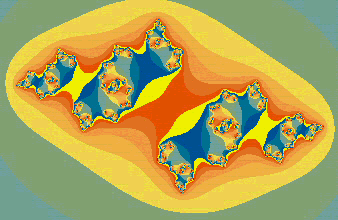
Jc being totally disconnected means that if A and B are in Jc, there is a disk around A
which hits no member of Jc and which excludes B. No Julia set ever breaks into two or more
disklike pieces to be connected without being totally disconnected. Given this fact and
the fact that the Jc have symmetry around the origin, it's not too surprising to learn
that Jc is connected if and only if the origin (0,0) is a member of Jc.
You can look at a lot of quadratic Julia sets in the CHAOS program by choosing the
Mandelbrot type and then using the Options menu to set the cursor type to select.
Every time you left click on the screen, it selects a value of c for a Jc. Right
clicking brings back the Mandelbrot set. Notice how the appearance of a Julia set
relates to the part of the Mandelbrot set you left click on.
The Quadratic Mandelbrot Set
If we think of varying c through all its complex values, we can think of a c-plane
which has a Jc set defined at each of its points. Benoit Mandelbrot had the idea of
looking at the locus of all the c's for which Jc is connected. This is the Mandelbrot set,
M. Symbolically,
M = { c : Jc is connected};
= { c : the origin is in Jc }, because Jc is connected iff (0,0) in Jc);
= { c : c is in Jc }, because if z0 = (0,0) then z1 = f(z0) = c.
= { c : c --fc--> FINITE }, by the definition of Jc.
The last definition of the Mandelbrot set corresponds to the way we actually compute
it. Each pixel position on the screen is identified with a distinct complex number c = u +
iv. We compute a COLORc for this value and set the pixel to that color. COLORc is computed
as follows. Set
z0 = c
z1 = c^2 + c
z2 = (c^2 + c)^2 + c = (z1)^2 + c
and so on, with the general step
zn+1 = (zn)^2 + c.
We repeat this step up to MAXITERATION times, where MAXITERATION is set as the program
parameter I. After each step we check the value of |zn| against a "large" value
BOUND. The value of BOUND which we use is the square root of seven. One can prove that if
|zn| passes BOUND, then |zn| will go on and get arbitrarily large as n increases. We also
keep track of the smallest value MINc which |zn| takes on, and we keep track of the value
of MINSTEPc at which MINc is hit.
If |zn| passes B for some value of n less than MAXITERATION, then we give the pixel a
color based on the value of n. We might take, for instance, COLORc = n MOD 16, where MOD
16 means "modulo 16," the remainder you would get if divided by 16. If |zn|
stays less than B for every value of n up through MAXITERATION, then we assume that the
pixel represents a point inside the Mandelbrot set. In the Blank fill method, we color
these points black. In the Bullseye fill method, we give such a pixel a color based on the
value of MINc. We might, for intstance, say COLORc = (1000 * MINc) MOD 16.

And in the Feathers fill method, we base the COLORc on the value MINSTEPc of the
iteration at which zn hits its smallest value, setting COLORc to something like MINSTEPc
MOD 16.
The Cubic Julia Sets
The maps which the Cubic Julias and Cubic Mandelbrots are based on have the form fkc,
with
fkc(z) = z^3 - 3*k*z + c. By translating the origin, any cubic map A*w^2 + B*w + C can
be put into the form w^3 - 3*k*z + c, with z a linear function of w. (The reason for
casting the linear coefficient in the form -3*k will be evident shortly.) For each fkc we
can define a cubic Julia set Jkc by:
Jkc = { z: z--fkc-->FINITE }.
Unlike in the quadratic case, these Julia sets are generally not symmetric. Some of
them are connected,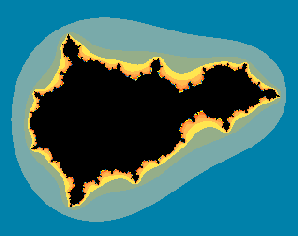
some are connected but not totally disconnected (made of numerous separate connected
patches),
and some are totally disconnected. It has been proved that Jkc is in fact connected if
and only if both the complex numbers k = a +ib and -k = -a -ib are in Jkc. As Jkc is not
symmetric, it may happen that only one of k or -k is in Jkc. Jkc is connected only when
both of these critical points are in Jkc.
Cubic Mandelbrot Sets
The four-dimensional set of all complex pairs k and c such that Jkc is connected is
known as the Cubic Connectedness map, or the CCM. This set has been studied by
Adrian Douady, John Hubbard and John
Milnor. [See Adrian Douady
and John Hubbard, "On the Dynamics of Polynomial-like Mappings", Annales
Scientifique de l'Ecole Normale Superieur 18:287.]
CCM = { (k,c) : Jkc is connected}; or
= { (k,c) : ( k --fkc--> FINITE ) AND ( -k --fkc--> FINITE ) }
The way our program depicts the CCM is to show various two-dimensional cross-sections
of it. These cross-sections are what we call Cubic Mandelbrot sets. If, for instance, k is
fixed, then we can look at the Cubic Mandelbrot set Mk.
Mk = { c : Jkc is connected};
= { c : ( k--fkc-->FINITE ) AND ( -k--fkc-->FINITE ) }.
In our software, the user has control of a cursor in the k-plane, meaning that each
cursor position selects a two dimensional value of k = a + ib. Whenever you press k, you
see Mk, the k-section of the cubic connectedness locus.
In CHAOS you can see a lot of cubic Mandelbrots and Julias as follows. Use the
Types dialog to set the type to Cubic Mandelbrot and use the Options dialog to set
the cursor type to select. Now left clicking will choose cubic Julias and right
clicking will choose cubic Mandelbrots. The right clicks choose the k values and the
left clicks choose the c values.
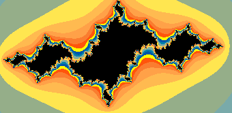
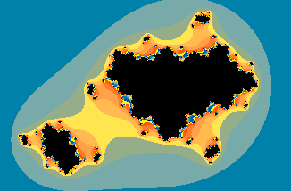
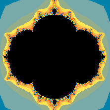
If k = 0+0i, one gets a degenerate Mk with fourfold symmetry; this is the default Cubic
Mandelbrot set.
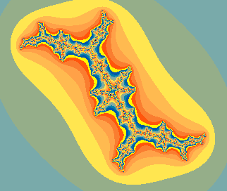
By slightly varying a and/or b, once can look at k-sections near each other, and try to
visualize stacking them one atop the other.
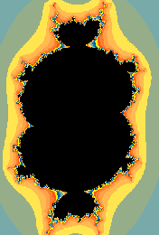
If |k| is large (about one or two), one gets an empty Mk. All the Mk have symmetry
around the origin, meaning that if c = u + iv is in Mk, -c = -u - iv will be in Mk, too.
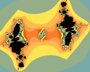
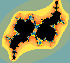
The appearance of the Mk is quite interesting. One often sees small replicas of the
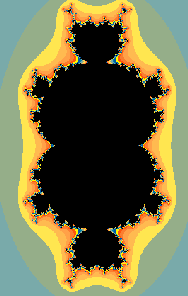
quadratic Mandelbrot set, though sometimes with wedges cut out of it. Looking at
successive sections, one often gets the impression of the Mk being like a cross-section of
a three-dimensional Mandelbrot shape, with buds all over it. But of course the full CCM is
four-dimensional, and this shows up in the fact that many of the bud cross-sections have
pieces missing from them. Presumably these missing pieces have inappropriate
four-dimensional coordinates for intersecting Mk.
As an aid to mathematical visualization, I think of it this way. The CCM is like a
three dimensional solid which is free to move pieces of itself to arbitrary time
locations. Thus if a section of a bud seems to have the right half missing, we might think
of the left half of the bud as being in Monday and the right half of the bud as being in
Tuesday, with your cross-section being computed at the Monday time coordinate. I use time
not at all in a physical sense here, but simply for the vividness of the image.
Now I explain how we compute Mk. The computation is done by fixing k = a + ib and then
varying c = x + iy and checking whether
k--fkc-->FINITE, and -k--fkc-->FINITE. On the basis of what I learn while doing
this checking, I will assign an Mk color(c) to the pixel representing c. Before starting,
I select a BOUND and a value of MAXITERATION, and say that k--fkc-->FINITE if for all n
less than MAXITERATION, the nth image of k is has norm less than BOUND. As before, we take
BOUND to be the square root of seven, and MAXITERATION can be set by the user.
Assuming k = a + ib has been set, our computation of the Mk color(c) for a fixed c = u
+ iv takes place as follows (this pseudocode description is not fully optimized):
initialize:
iteration = 0;
tx = a;
ty = b;
a3 = -3 * ( a * a - b * b );
b3 = -3 * ( 2 * a * b );
and then iterate:
x2 = tx * tx;
y2 = ty * ty;
xa = x2 - y2 + a3;
yb = 2*tx*ty + b3;
temp = xa * tx - yb * ty + u;
ty = xa * ty + yb * tx + v;
tx = temp;
iteration = iteration + 1;
until x2 + y2 > BOUND or iteration = MAXITERATION, saving
iteration as iteration1;
and then reinitialize
iteration = 0;
tx = -a;
ty = -b;
a3 = -3 * ( a * a - b * b );
b3 = -3 * ( 2 * a * b );
and iterate the same computation,
until x2 + y2 > BOUND or iteration = MAXITERATION, saving
iteration as iteration2;
If iteration1 and iteration2 both equal MAXITERATION, then
Mk color(c) = 0.
Otherwise,
Mk color(c) = min(iteration1,iteration2).
As well as the cubic Mk CCM cross-sections, we can also compute
Mc = { k : Jkc is connected};
= { k : ( k--fkc-->FINITE ) AND ( -k--fkc-->FINITE ) }.
The Mc are, to my eye, not as interesting as the Mk. But you can look at them in
CHAOS and decide for yourself. You can get them by going to the Option menu and
selecting the 4D Slice to be AB instead of UV. The other slice options represent
different possible plane slices through the CCM.
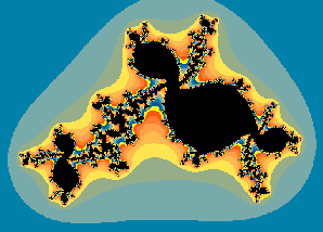
The "Rudy Set"
An apparently new fractal which I have enjoyed investigating is this.
R = {k : k is in Mk}
= {k : Jkk is connected}
= {k : ( k --fkk--> FINITE ) AND
( -k
--fkk--> FINITE) }.
I immodestly call it the Rudy set!
Compare the definition of R as { k : k is in Mk } to the definition of M as { c : c is
in Jc }.
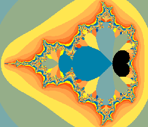
R is an object which is extremely rich in fractal structures. One good region is
the plume between 2 and 3 o'clock. I call this area "Mars". 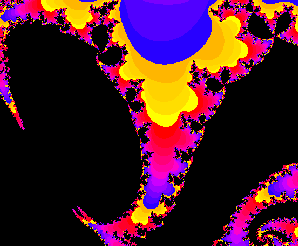
The Rhorse image that forms the background tile for this and the CHAOS page is found in
the Mars region of the Rudy set. Another good region is the spike at the top, at 12
o'clock. There is an interesting structure there that is a bit like a Mandelbrot
set, but different.
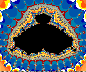
You can view this set with CHAOS.
I used to think there would be an an alternate form of the Rudy set definable as
R' = {c : c is in Mc}. But this would just be {c : Jcc is connected}, which is the
same as R.
Further Directions
A set which I am interested in computing (though I have not yet done so) is
NZK = {k : Mk is non-empty}.
To compute NZK, I would have to step k = a + ib through every onscreen value (a and b
might range from -1.5 to 1.5), and for each of these k run the computation of Mk until at
least one pixel is colored black. If any pixel of Mk is colored black during the
computation of Mk, then k is a member of NZK and I color k black.
The value of computing NZK and having it to hand as a .GIF file is that then, I
would know where to put my cursor so as to select k values to get full or nearly empty Mk
graphs. The most exotic Mk graphs probably occur for k values near the boundary of NZK,
just as the more interesting Julia sets Jc occur at c values that are near the boundary of
M.
As an extension of the set NZK, I would also like to map a coloring of the k-plane in
which the color at k is a linear function of the relative pixel area of Mk. To compute the
relative pixel area of Mk, I set in motion a computation of Mk at some pixel resolution.
Suppose for instance that I am going to compute P# pixels. Now if Bk# is the number of
pixels which are assigned the black color during the computation of Mk, then the relative
pixel area of Mk is said to be equal to Bk#/P#. Presumably the Mk are measurable, and the
relative pixel area of each Mk converges to a precise limit as #P is increases. In
practice, I will first compute the relative pixel count map by simply running each Mk
computation for each pixel in the upper half plane ( due to symmetry, the count in the
lower half plane is identical), and then defining K color(k) to be, say, Bk# MOD maxcolor.
The value of the relative pixel area map of the k-plane would be that if one wants to
stack 2D cross-sections up to get a nice looking 3D object, it would probably be a good
idea to have the change in area between successive slices be minimal. This could be done
by choosing your k along a level path in the R-color map. Alternatively, choosing k along
the gradient or "steepest descent" path of maximal area change might be
interesting as well! |