


Figure 1: The CAPOW! Color dialog box, showing the color map used in the following figures.
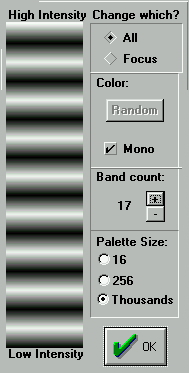 Figure 1.
In the CAPOW! experiments to be discussed here, we will be looking at
one-dimensional cellular automata. The arrays are about two hundred cells
wide, and we use periodic boundary conditions, wrapping the left end to
match the right end. In order to view the activity in a given CA, we show
two different views of the CA, as in Figure 2. The lower part of the figure
shows an instantaneous image of the CA in the form of a graph of cell intensity
against cell position. The upper part of the figure shows a space-time
diagram of the CAs history of states, with the time axis running from top
to bottom. In the space-time diagram, each instantaneous state of the CA
is represented as a single horizontal line, with the pixel colors being
based on the intensity at the corresponding cell position. The earlier
CA states correspond to horizontal lines higher up in the image, and the
bottom line of the image corresponds to the CA state currently being displayed
as a graph. Figure 2 shows the stable wave equation simulation scheme (31a),
seeded by a randomly chosen Fourier sum of several sine waves. The value
of  used is 0.02, the value
of
used is 0.02, the value
of  used is 0.024, and
the clamping range is -150.0 to 150.0. Wave equation simulations are not
particularly sensitive to these values, as long as one is sure that
used is 0.024, and
the clamping range is -150.0 to 150.0. Wave equation simulations are not
particularly sensitive to these values, as long as one is sure that  is greater than
  , and that
the initial seed values chosen lie within the clamping range.
, and that
the initial seed values chosen lie within the clamping range.
Figure 2: The wave equation simulation, seeded by a Fourier sum of sine waves.
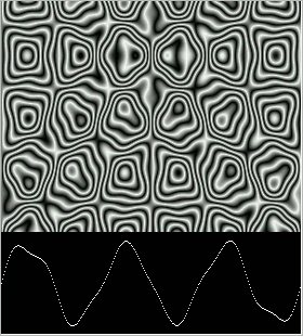 Figure 2.
It is possible to show several CAs at once in CAPOW! Figure 3 shows the results of seeding the wave simulations with, clockwise from upper left, a single tent-peak, a sine wave, a Fourier sum, and random values. The sine wave seed yields a space-time pattern that looks a bit like a box of sushi. The random seed does not settle down for the linear wave scheme.
Figure 3: The wave equation seeded by a spike, Wave, Fourier Sum, and Random noise.
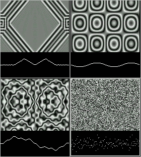 Figure 3.
We discussed the issue that the space step must be greater than or equal to the time step. Experiment shows the simulation to be more robust if it is strictly greater. As mentioned before, if we do set the space step equal to the time step, the scheme reduces to scheme (31a*). In Figure 4 we show how this rule can lead to an alternating pattern.
Figure 4 below was arrived at by seeding the CA with a sine wave, and by then introducing a step-discontinuity at a small interval overlapping the left and right boundaries (recall that we use periodic boundary conditions.) More precisely, we patch in a small interval of values taken from a sine wave of a different phase.
When the perturbation first happens, we see a pattern like in the middle of the spacetime picture, with the disturbance moving inward from both the left and the right ends. As the CA continues to evolve, the two perturbation waves repeatedly pass through each other at the center of the CA, proceed out to the ends, wrap around to move back towards the center and so on. Figure 4 shows the CA after it has already undergone several of these cycles since the initial perturbation event. If left alone, the CA will repeat this pattern indefinitely.
When we refer to the CA in Figure 4 as having an ``alternating" pattern
of instability, we mean that the odd-numbered and the even-numbered cells
are out of step with each other. If the  were strictly greater than the
  in Figure 4, the image would change in two ways: the upper left and lower
right rows of dots would be vertically translated so as to lie evenly with
the rest of the curve; and the spacetime diagram part would be less fuzzy.
The perpetually criss-crossing perturbation pattern would remain.
in Figure 4, the image would change in two ways: the upper left and lower
right rows of dots would be vertically translated so as to lie evenly with
the rest of the curve; and the spacetime diagram part would be less fuzzy.
The perpetually criss-crossing perturbation pattern would remain.
Figure 4: An unstable wave, with the odd space-time cells out of phase with the even space-time cells.
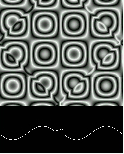 Figure 4.
Now let's turn to the Quadratic Nonlinear Wave based on scheme (34). First note that this simulation very easily becomes unstable. If we set the nonlinearity to 0.385 and seed it with a Fourier seed, we see a result like in Figure 5. The simulation breaks down and becomes unstable at several points, and the breakdowns spread at the speed of the wave in the medium. In order to avoid floating point overflow, we clamp our maximum and minimum wave values to be in a certain range (-12.0 to 12.0 in the case of Figure 5). A result of this is that the cell values spend a lot of time at the maximum and/or minimum values. Because these special values are visited so often, certain intermediate values calculated from these special values are visited often as well. This has the effect of making the continuous CA behave somewhat like a discrete-valued CA with a limited number of states. Note in Figure 5 how the unstable zone shows behavior similar to discrete-valued CA. In terms of Wolfram classification, this CA seems to be of the glider-sustaining type 4, as evidenced by the zig-zagging patterns which send off diagonal lines.
Figure 5: Quadratic Nonlinear Wave Breakdown, Nonlinearity 0.385
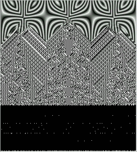 Figure 5.
For the rest of our Quadratic Nonlinear Wave experiments we use these
parameters:  is 0.109,
  is 0.090, the clamping range for U is -12.0 to 12.0, and the
  ``quadratic nonlinearity" value in scheme (35) is 0.076.
For our first experiment with these settings, we seed the CA with a random selection of values. Due to instability, the CA values get repeatedly clamped, producing an appearance like a discrete-valued type 4 CA, as shown in Figure 7. For this particular value of the nonlinearity parameter, the repeated clampings of the CA happen to bring groups of cells into approximate continuity, and the CA then evolves into a smooth pattern marked by step-shaped waves and a single maximal discontiunity as shown in Figures 8 and 9. For lower values of the nonlinearity parameter, there is not enough clamping to impose this artificial continuity, while for higher values of the nonlinearity parameter, the imposed continuity takes over to make the CA cell values constant across the entire space. From a CA standpoint these patterns are interesting, although from a physical standpoint they are simply artifacts of a broken simulation.
Figures 6, 7, 8: A clamped quadratic nonlinear wave seeded with random values evolves into something smooth.
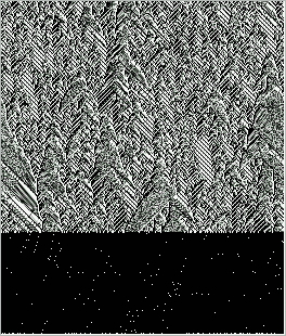 Figure 6.
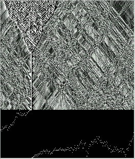 Figure 7.
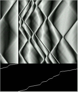 Figure 8.
The Fermi, Pasta, and Ulam paper [2] reports on experiments carried out by seeding schemes based on the quadratic and cubic forms of the nonlinear wave equation with a sine wave, and then repeatedly examining the power spectrum (i.e., Fourier modes) of the shape assumed by the ``nonlinear string" as more and generations go by.
In his autobiography, Ulam gave a nice summary of the surprising results of some of their experiments,
``It was the consideration of an elastic string with two fixed ends, subject not only to the usual elastic force of strain proportional to strain, but having, in addition, a physically correct small nonlinear term. The question was to find out how this nonlinearity after very many periods of vibration would gradually alter the well-known periodic behavior ... and how, we thought, the entire motion would ultimately thermalize, imitating perhaps the behavior of fluids which are initially laminar and become more and more turbulent. ... The results were entirely different qualitatively from what even Fermi, with his great knowledge of wave motions, had expected. The original objective had been to see at what rate the energy of the string, initially put into a single sine wave ... would gradually develop higher tones with the harmonics, and how the shape would finally become `a mess' ... To our surprise the string started playing a game of musical chairs, only between several low notes, and ... came back almost exactly to its original sinusoidal shape." [11], pp. 226-227.
CAPOW! confirms the behavior Ulam observed for both the quadratic and the cubic forms of the nonlinear term.
In Figures 9 through 16, we look at the long-term evolution of a nonlinear Quadratic CA seeded with a sine wave. The time step counts given are approximate; the behavior does not change rapidly enough for greater precision to be required. We might mention here that on a Pentium machine running a single CA of about two hundred cells wide, CAPOW! does about one hundred complete CA updates per second, and you can run a hundred thousand steps in about fifteen minutes. Because the quadratic scheme is not spatially symmetric, the sushi wave patterns become pointed. When observed running, the moving graph of the CA produces an illusion of rotation. The rotation effect centers on the vertices where the longer pieces of the curve connect the shorter pieces, as in Figures 9, 10, and 11. These vertices, which correspond to the maxima and minima of the original sine-wave seed, seem to rotate clockwise around the points at the centers of the segments, which correspond to the initial seed values of 0. As the vertices approach and recede from each other, the connecting segments look as if they are being squashed and stretched, with secondary waves being sent off from the ``rotating" tips.
Figure 9: Quadratic Wave after 100 steps.
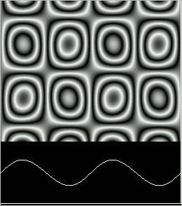 Figure 9.
Figure 10: Quadratic Wave after 1,500 steps.
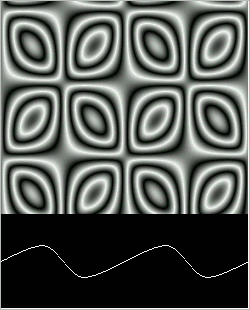 Figure 10.
Figure 11: Quadratic Wave after 3,000 steps.
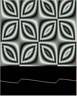 Figure 11.
As the evolution continues, higher frequency terms are produced by the perturbations caused by the stretching and shrinking of the wave. The pattern remains periodic. After about a million iterations a pattern similar to the starting pattern seems briefly to reemerge.
Figure 12: Quadratic Wave after 6,000 steps.
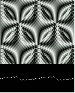 Figure 12.
Figure 13: Quadratic Wave after 12,000 steps.
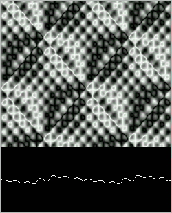 Figure 13.
Figure 14: Quadratic Wave after 30,000 steps.
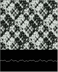 Figure 14.
Figure 15: Quadratic Wave after 42,000 steps.
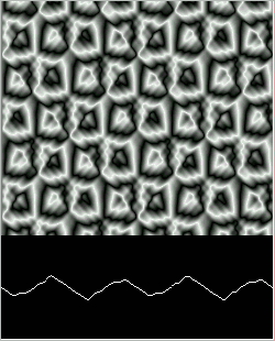 Figure 15.
Figure 16: Quadratic Wave after 100,000 steps.
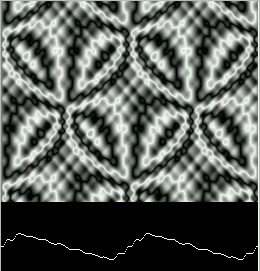 Figure 16.
The reemergence of the seed wave happens even more clearly for the cubic form than for the quadratic form of the nonlinear wave simulation.
For our Quadratic Nonlinear Wave experiments we use these parameters:  is 0.109,
  is 0.090, the
clamping range for U is -1.0 to 1.0, and the
is 0.090, the
clamping range for U is -1.0 to 1.0, and the  ``cubic nonlinearity" value in scheme (36) is 10.720.
Because of the scheme's left-right symmetry, the cubic scheme is less apt to break down than is the quadratic scheme, so we can set the nonlinearity to a fairly large value. On the other hand, cubing a number greater than one can greatly amplify it, which is why we restrict our intensities to the range -1.0 to 1.0.
We seed the cubic wave with a sine wave. The nonlinear effects of the scheme show themselves more slowly than in the quadratic case. The first effect visible is a bending of the sushi into badge shapes, with the wave becoming pointy instead of smooth. Soon secondary points occur, with the peaks of the wave folding down while the sides are still moving up. Increasingly complicated, but still periodic, patterns occur.
Figure 17: Cubic Wave after 100 steps.
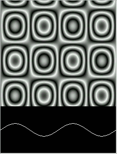 Figure 17.
Figure 18: Cubic Wave after 6,000 steps.
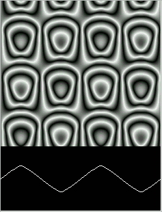 Figure 18.
Figure 19: Cubic Wave after 24,000 steps.
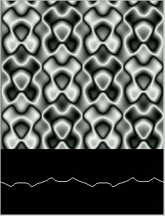 Figure 19.
Figure 20: Cubic Wave after 36,000 steps.
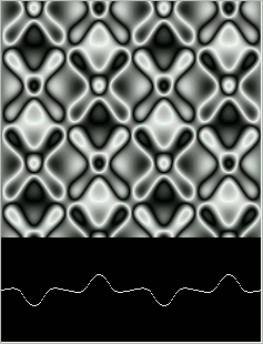 Figure 20.
Finally a kind of maximum level of ``thermalization" is obtained with most of the wave's energy in low amplitude high frequency oscillations, as in Figure 21.
Figure 21: Cubic Wave after 48,000 steps.
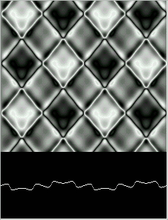 Figure 21.
Now the return begins. Slowly the evolution of the wave retraces itself, eventually getting back to something very much like the initial condition.
In the quadratic case, Zakharov [12] has explained this quasiperiodic behavior for the differential equation being simulated (eq (8)). Recently, Bukowski [13] has used Sobolev estimates to expand Zakharov's results to explain this quasiperiodic behavior for the discrete simulations presented here. Proof of the quasiperiodicity in the cubic case has not yet been established, though it seems likely to have an explanation that parallels the quadratic case.
Figure 22: Cubic Wave after 90,000 steps.
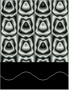 Figure 22.
Figure 23: Cubic Wave after 120,000 steps.
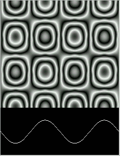 Figure 23.